In this project, my team decided to deep dive into the mortgage rates in New York pre, during, and post pandemic of the Covid-19 Virus. We aimed to see that if the county you live in, income you make, and demographics you identify with affect mortgage loans and rates through these stages.
Data Sources
To do this, we narrowed down our resources to two main data sources.
First, we decided to pull data from the Consumer Finance Protection Bureau- HMDA Data. From this data, we retrieved the loan type, loan amount, interest rate, and much more. Alex retrieved this data.
Second, we decided to pull data from the United States Census Bureau. From this data, we retrieved mean income, population by race, job distribution, and much more. I was in charge of retrieving this data, and I will explain how I did so below.
I used two files from the Census Bureau to get the necessary data we needed:
My contribution to this project began with retrieving data from the Census Bureau. The first thing I had to do was retrieve a personal key to access the database. Then, I downloaded the tidycensus library into my Rstudio, as well as the following libraries. This can be seen in the folded code below.
Click here to see how the libraries were downloaded
Installing package into 'C:/Users/laure/AppData/Local/R/win-library/4.4'
(as 'lib' is unspecified)
package 'plyr' successfully unpacked and MD5 sums checked

The downloaded binary packages are in
    C:\Users\laure\AppData\Local\Temp\Rtmp8oHmZ7\downloaded_packages
── Conflicts ────────────────────────────────────────── tidyverse_conflicts() ──
✖ dplyr::filter() masks stats::filter()
✖ dplyr::lag()    masks stats::lag()
ℹ Use the conflicted package (<http://conflicted.r-lib.org/>) to force all conflicts to become errors
Warning: package 'tigris' was built under R version 4.4.2
To enable caching of data, set `options(tigris_use_cache = TRUE)`
in your R script or .Rprofile.
library(ggplot2)library(sf)
Warning: package 'sf' was built under R version 4.4.2
Linking to GEOS 3.12.2, GDAL 3.9.3, PROJ 9.4.1; sf_use_s2() is TRUE
library(plotly)
Warning: package 'plotly' was built under R version 4.4.2
Attaching package: 'plotly'

The following object is masked from 'package:ggplot2':

    last_plot

The following object is masked from 'package:stats':

    filter

The following object is masked from 'package:graphics':

    layout
library(gganimate)
Warning: package 'gganimate' was built under R version 4.4.2
library(viridis)
Warning: package 'viridis' was built under R version 4.4.2
Loading required package: viridisLite
library(scales)
Warning: package 'scales' was built under R version 4.4.2
Attaching package: 'scales'

The following object is masked from 'package:viridis':

    viridis_pal

The following object is masked from 'package:purrr':

    discard

The following object is masked from 'package:readr':

    col_factor
Your original .Renviron will be backed up and stored in your R HOME directory if needed.
Your API key has been stored in your .Renviron and can be accessed by Sys.getenv("CENSUS_API_KEY").
To use now, restart R or run `readRenviron("~/.Renviron")`
[1] "fd444ca335bf9020633084575dbe45c1529be65f"
# Combined_Data can be found on Ayrat's Repo and be readily downloaded. combined_data <-readRDS("C:/Users/laure/OneDrive/Desktop/combined_data.rds")
After this, I began to download the data in the following manners.
Downloading & Cleaning the Data
First, to clean the data, I created a table to change the variables to make the data easier to read, as the data was only identifiable by the nine digit code assigned to it.
Click here to see how the variables were changed
vars_2018 <-load_variables(2018, "acs1", cache =TRUE)var_map <-c("B02001_001"="Estimated Total","B02001_002"="White Alone", "B02001_003"="Black or African American Alone", "B02001_004"="American Indian and Alaska Native Alone","B02001_005"="Asian Alone", "B02001_006"="Native Hawaiian and other Pacific Islander Alone","B02001_007"="Some Other Race", "B02001_008"="2 or more races")
Then, I downloaded all of the data into my R, from 2018 - 2023. Notice that the data from 2020 is unavailable. This is due to the pandemic not giving reliable data, so the Census does not readily offer it in the same fashion.
To retrieve the data, I used the tidycensus library to pull from the Cenus’ records. I then picked what variables I want from the data, and put what year I wish to pull. After, I filtered the data to only show the New York counties, rather than the entire United States. Lastly, I renamed the columns and changed the variable names to make the data set easier to read. I repeated this process for the following desired years.
Click here to see how the population data was downloaded into R
Next, I wanted to create a table to show all of the populations through the years, by race and county. To do this, I joined the table with the code below, on the items of GEOID and race.
Click here to see how the data was joined
total_population_race <- population_1901_2018 |>left_join(select(population_1901_2019, y2019, GEOID, race), by =c("GEOID", "race")) |>left_join(select(population_1901_2021, y2021, GEOID, race), by =c("GEOID", "race")) |>left_join(select(population_1901_2022, y2022, GEOID, race), by =c("GEOID", "race")) |>left_join(select(population_1901_2023, y2023, GEOID, race), by =c("GEOID", "race"))
The data table can be viewed below.
datatable(total_population_race)
Now that this data was retrieved, I moved on to the data that shows the mean household income by county. This retrieval can be seen below. I retrieved the information the same way I retrieved the population amount by race above.
This can be seen below in the folded code.
Click here to see how the data was downloaded into R and cleaned
Then, I created a data table to show all of the households from 2018-2023, by income and county.
Click here to see how this was done
# Join tablestotal_income_household <- Income_2018 |>left_join(select(Income_2019, y2019, GEOID, income), by =c("GEOID", "income")) |>left_join(select(Income_2021, y2021, GEOID, income), by =c("GEOID", "income")) |>left_join(select(Income_2022, y2022, GEOID, income), by =c("GEOID", "income")) |>left_join(select(Income_2023, y2023, GEOID, income), by =c("GEOID", "income"))
This data table can be viewed below.
datatable(total_income_household)
Thirdly, I decided to download the mean income per capita per race by county. which can be seen in the folded code below. This was done the same way as above.
Click here to see how the data was downloaded into R and cleaned
# Mean Incomes per capita var_map3 <-c("S1902_C03_001"="All Household Income Mean","S1902_C03_020"="White Alone", "S1902_C03_021"="Black or African American Alone", "S1902_C03_022"="American Indian and Alaska Native Alone","S1902_C03_023"="Asian Alone", "S1902_C03_024"="Native Hawaiian and other Pacific Islander Alone","S1902_C03_025"="Some Other Race", "S1902_C03_026"="2 or more races")# Get 2018mean_income_2018 <-get_acs(geography ="county",variables =c("S1902_C03_001E", "S1902_C03_020E", "S1902_C03_021E", "S1902_C03_022E", "S1902_C03_023E", "S1902_C03_024E", "S1902_C03_025E", "S1902_C03_026E"),year =2018,survey ="acs1")
Getting data from the 2018 1-year ACS
The 1-year ACS provides data for geographies with populations of 65,000 and greater.
Data table that shows all of the households from 2018-2023, by income and county.
Click here to see how this was done
# Join tablestotal_mean_incomes <- mean_income_2018 |>left_join(select(mean_income_2019, y2019, GEOID, race), by =c("GEOID", "race")) |>left_join(select(mean_income_2021, y2021, GEOID, race), by =c("GEOID", "race")) |>left_join(select(mean_income_2022, y2022, GEOID, race), by =c("GEOID", "race")) |>left_join(select(mean_income_2023, y2023, GEOID, race), by =c("GEOID", "race"))
This data table can be viewed below.
datatable(total_mean_incomes)
Lastly, I pulled data to show the population per occupation type by county. The following is how the data was downloaded, again, similar to how it was done above.
Click here to see how the data was downloaded into R and cleaned
# Join tablestotal_occupations <- main_occupation_2018 |>left_join(select(main_occupation_2019, y2019, GEOID, job_type), by =c("GEOID", "job_type")) |>left_join(select(main_occupation_2021, y2021, GEOID, job_type), by =c("GEOID", "job_type")) |>left_join(select(main_occupation_2022, y2022, GEOID, job_type), by =c("GEOID", "job_type")) |>left_join(select(main_occupation_2023, y2023, GEOID, job_type), by =c("GEOID", "job_type"))
The data table can be viewed below.
datatable(total_occupations)
Now that I retrieved all of the data needed, I decided to format each of the tables in a different way so it would be easier to run the code. Thus, I put the tables into a long format. Now, when I attempt to create facet maps or make judgement by year, I will not run into any issues. This can be seen below.
All of the tables seen below will be the ones I contributed to our group project. Since I was in charge of our data on a geographic level, this is the majority of what my work amounted to.
I sought out to solve the following questions:
What is the mean income amount by county?
What is the total loan amount by county?
What are the main jobs/occupations by county?
My graph was prepared with the following code below.
`summarise()` has grouped output by 'county_code', 'NAME'. You can override
using the `.groups` argument.
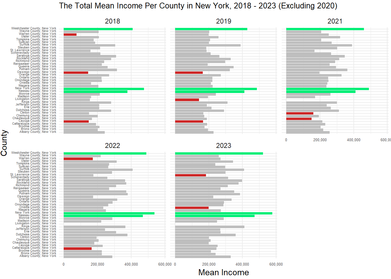
total_loan <- total_loan |>rename(year = activity_year) |>mutate(year =as.numeric(year),county_code =as.numeric(county_code))total_loan_mean_income <- total_mean_incomes_long22 |>inner_join(total_loan, by =c("county_code", "year"))total_loan_mean_income2 <- total_loan_mean_income |>group_by(year) |>mutate(Highlight =case_when( Total_loan %in%sort(Total_loan, decreasing =TRUE)[1:3] ~"Highest", Total_loan %in%sort(Total_loan, decreasing =FALSE)[1:3] ~"Lowest",TRUE~"Normal" ))total_loan_mean_income3 <- total_loan_mean_income |>group_by(year) |>mutate(Highlight =case_when( mean_income %in%sort(mean_income, decreasing =TRUE)[1:3] ~"Highest", mean_income %in%sort(mean_income, decreasing =FALSE)[1:3] ~"Lowest",TRUE~"Normal" ))income_plot <-ggplot(total_loan_mean_income3, aes(x = NAME, y = mean_income, fill = Highlight)) +geom_bar(stat ="identity", show.legend =FALSE) +scale_fill_manual(values =c("Highest"="springgreen2", "Lowest"="firebrick3", "Normal"="gray")) +facet_wrap(~year) +coord_flip() +labs(title ="The Total Mean Income Per County in New York, 2018 - 2023 (Excluding 2020)", x ="County", y ="Mean Income") +theme_minimal() +theme(plot.title =element_text(size =10),axis.text.y =element_text(size =4, vjust =0, margin =margin(r =1)),axis.text.x =element_text(size =5),plot.margin =margin(3, 3, 3)) +scale_y_continuous(labels =label_comma())
plot(income_plot)
This plot showed how the total mean income per county changed overtime. The three highest counties are represented by the green bars and the three lowest by the red bars. Here we can see that the three highest paid counties remained the same over the 6 years, being Westchester County, New York County, and Nassau county. On the other hand, the three lowest mean income counties fluctuated overtime, but remotely stayed consistent. Incomes seemed to stay consistent over the years, with slight growths occurring after Covid.
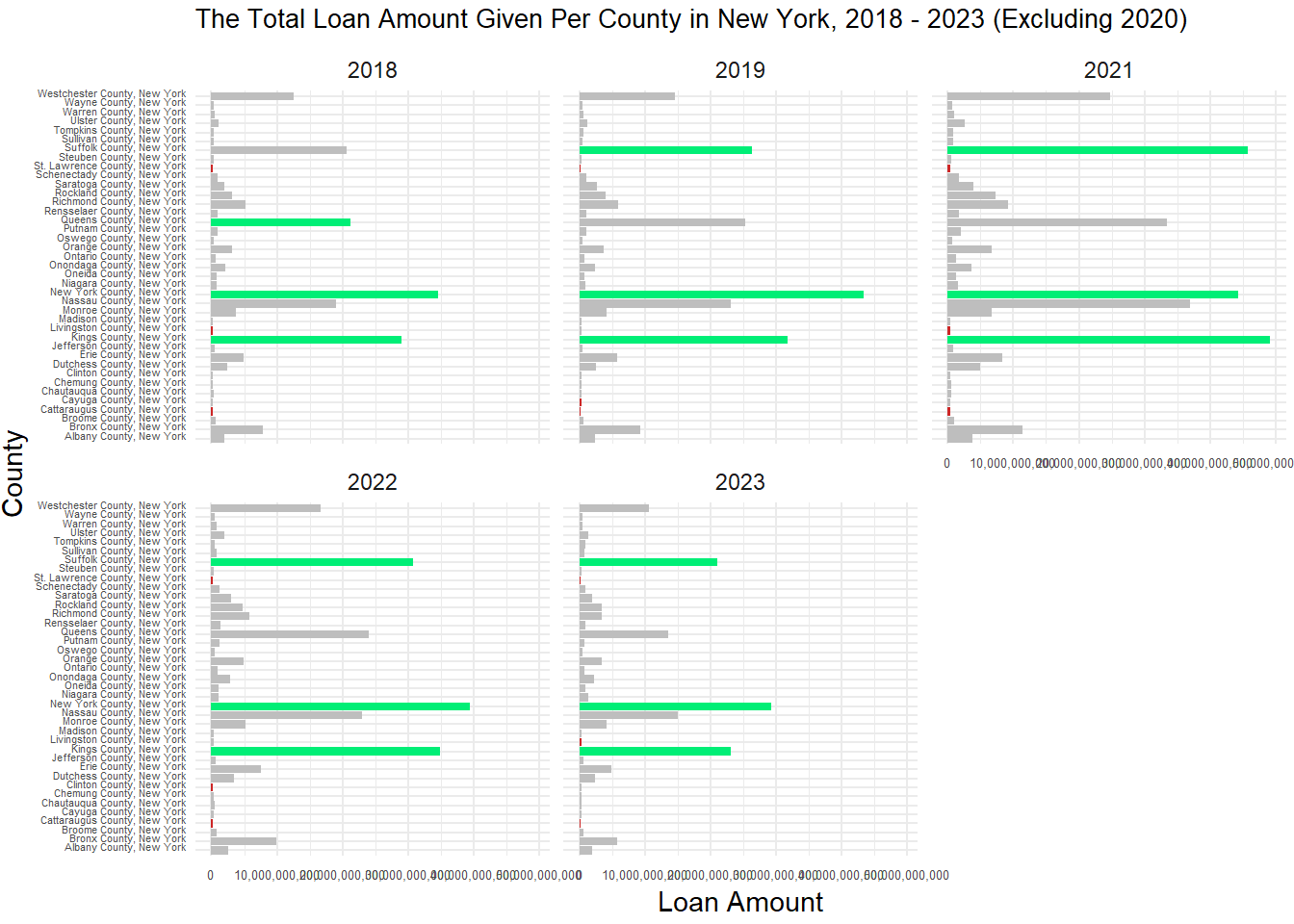
Next, I looked into the Total Loan by County. This can be seen below.
Click here to see how this was done
loan_plot <-ggplot(total_loan_mean_income2, aes(x = NAME, y = Total_loan, fill = Highlight)) +geom_bar(stat ="identity", show.legend =FALSE) +scale_fill_manual(values =c("Highest"="springgreen2", "Lowest"="firebrick3", "Normal"="gray")) +facet_wrap(~year) +coord_flip() +labs(title ="The Total Loan Amount Given Per County in New York, 2018 - 2023 (Excluding 2020)", x ="County", y ="Loan Amount") +theme_minimal() +theme(plot.title =element_text(size =10),axis.text.y =element_text(size =4, vjust =0, margin =margin(r =1)),axis.text.x =element_text(size =5),plot.margin =margin(3, 3, 3)) +scale_y_continuous(labels =label_comma())
plot(loan_plot)
This plot depicts the total loan amount per county over time. Again, the green represents the three highest and the red represents the lowest. Here, we can see that besides 2018, the three highest counties remained the same. The three lowest remained consistent, but not exactly the same. It is also important to realize that the counties that tended to have the lower incomes also had the lower total loan amount given and the highest incomes tended to receive the highest total loans. It is also important to note that after Covid, each county received less total loan amounts than they did before Covid.
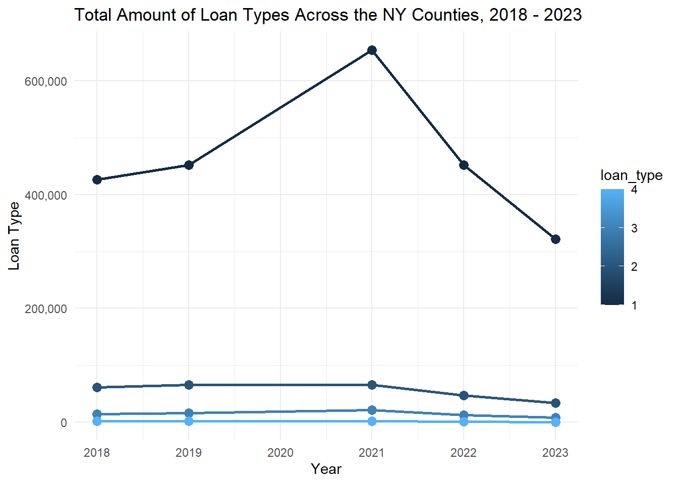
For my third plot, I looked into the total loan types over time. I wanted to see if all of the loans were affected by Covid. This can be seen below.
`summarise()` has grouped output by 'county_code', 'NAME'. You can override
using the `.groups` argument.
pop_loan <- combined_data |>select(activity_year, county_code, loan_type) |>group_by(county_code, activity_year) |>mutate(activity_year =as.numeric(activity_year),county_code =as.numeric(county_code))pop_loan_count <- pop_loan |>group_by(county_code, activity_year, loan_type) |>summarize(count =n(), na.rm =TRUE, .groups ='drop') |>rename(year = activity_year)count_loan_mean_income <- total_mean_incomes_long22 |>inner_join(pop_loan_count, by =c("county_code", "year"))top_loan <- count_loan_mean_income |>group_by(county_code, NAME, year) |>arrange(desc(count))sum_loans <- top_loan |>group_by(loan_type, year) |>summarize(total_count =sum(count), .groups ="drop")top_loan_plot <-ggplot(sum_loans, aes(x = year, y = total_count, color = loan_type, group = loan_type)) +geom_line(size =1) +geom_point(size =3) +labs(title ="Total Amount of Loan Types Across the NY Counties, 2018 - 2023" , x ="Year", y ="Loan Type") +theme_minimal() +scale_y_continuous(labels =label_comma())
Warning: Using `size` aesthetic for lines was deprecated in ggplot2 3.4.0.
ℹ Please use `linewidth` instead.
plot(top_loan_plot)
This graph shows the four types of loans compared over the years, with lines representing the total from every county. Here, it can be seen that loan type 1 is by far the most frequent loan type of the four. We can also see that after the height of Covid struck in 2021, each loan type experienced a drop, with loan type one experiencing the most dramatic drop.
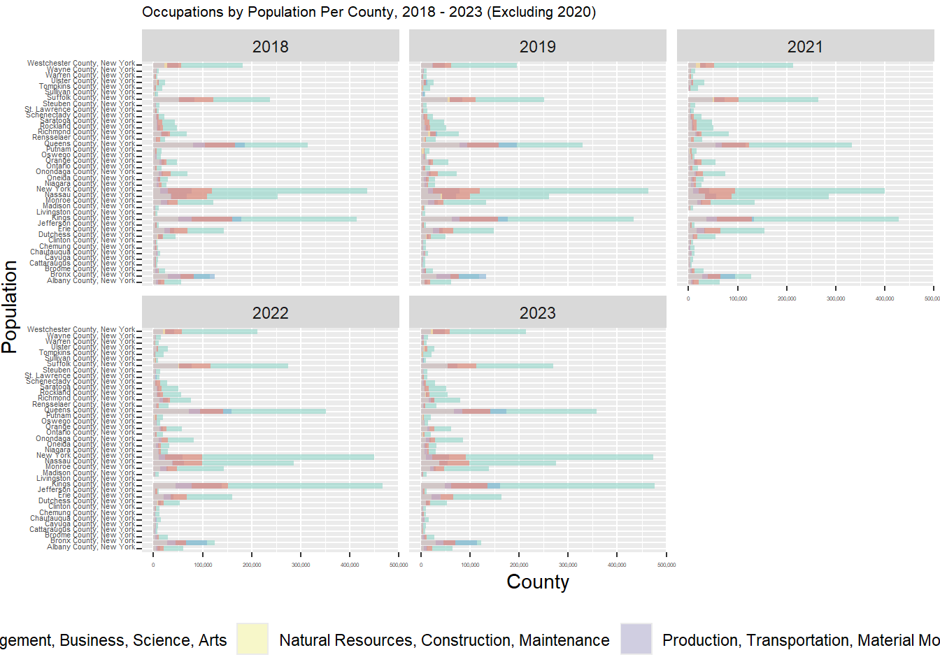
Lastly, I looked into the total populations per occupations by county, over time. This can be seen below.
Click here to see how this was done
occupations <- total_occupations_long |>filter(!apply(total_occupations_long, 1, function(row) any(grepl("Total Employed Full-Time", row, ignore.case =TRUE))))occupations_plot <-ggplot(occupations, aes(x = NAME, y = population, fill = job_type)) +geom_bar(stat ="identity", position ="identity", alpha = .6, width = .9) +facet_wrap(~year) +coord_flip() +labs(title ="Occupations by Population Per County, 2018 - 2023 (Excluding 2020)", y ="County", x ="Population") +theme(legend.position ="bottom", plot.title =element_text(size =8),axis.text.y =element_text(size =4, vjust =0, margin =margin(r =1)),axis.text.x =element_text(size =3),plot.margin =margin(3, 3, 3)) +scale_fill_brewer(palette ="Set3") +scale_y_continuous(labels =label_comma())
plot(occupations_plot)
Warning: Removed 20 rows containing missing values or values outside the scale range
(`geom_bar()`).
Above is a graph we derived from our data to show occupation by county. Interestingly enough, we can see that the “Management, Business, Science, Arts” category dominated the four other categories in every single county.
Overall Findings
Does the county you live in affect how much money you make?
Yes, the county you live in does affect how much you make, as some make progressively more than others
Does the mean income that a county makes correlate with the total amount of loans a county receives?
Yes, they do correlate. The counties that tended to have lower mean incomes, had less total loans. The ones that had a higher mean income, had more total loans.
Did any change occur with mean income and total loans before, during, and after COVID?
Mean income seemed to get higher after COVID in each county, while the Total Loans seemed to get lower. For both, the highest counties remained the same while the lowest counties varied throughout the years.
Was there a loan type that prevailed over the others, and did the total loans given change overtime?
Yes, Loan Type 1, Conventional Loans, was the highest in each county by far. After 2021, each loan type experienced a dramatic drop.
Was there a job category that prevailed in each county overtime?
Yes, the Management, Business, Science, Art category prevailed in each county overtime by far.
Conclusion
Therefore, my contribution to this project resided mostly in retrieving the data from the Census, cleaning/creating the necessary tables, and conducting the analysis on our data at a geographic level. For the written part of the project, I also contributed greatly in both presentations and the final written group report. Everything else was completed by my lovely group members.